
|
| |||
|
|
|||
|
Current distribution calculations Antenna design and simulations Sensor modeling Current distributions on metallic plates Inverse scattering simulations Experimental inverse scattering
|
Formal Compensation of Sensor-Related Interaction for Iterative Inverse ScatteringThis research page presents a contribution to the development of free-space microwave imaging algorithms. A formal compensation method of sensor-related interactions is presented. The microwave imaging problem is an inverse scattering problem in which, from the measurement of the scattered field from a test object, the dielectric contrast distribution with respect to the external medium is reconstructed. Generally, the measurement system perturbations are not explicitly taken into account for the modeling. At most, a linear relation is assumed between the measured field by the sensors and the field in which it is placed. This work shows that in many cases it is necessary to take into account all the interactions in the reconstruction formalism, including the ones related to the measurement system. The starting point of the analysis is the electric field integral equation from which the so-called coupling and observation discretized equations are derived by application of the method of moments. It is shown that the introduction of an equivalent scattered field allows transformation of these two equations in order to get back to the case in which the sensor-related interactions are neglected.
The reconstruction process is based on the Newton-Kantorovich method in which,
from an initial distribution of the dielectric contrast, the difference between
the measured and model-computed equivalent scattered fields is minimized. This
formalism is presented for the two-dimensional scalar case and has been
successively extended to the scalar and vector three-dimensional cases. The
modeling of two experimental microwave imaging systems has been performed: one
for medical imaging and the other for free-space dielectric characterization.
Forward Scattering Simulations
In the Newton-Kantorovich method, a forward scattering problem needs to be
solved at each iteration, using updated values of the contrast of the object
to be reconstructed.
The first keypoint of the formal compensation method is therefore to accurately
model the scattering problem by taking into account the sensors' perturbation.
In the following, the sensors are either assumed to be metallic wires (2D model)
or quarter wavelength dipoles (3D model). Figure 1 shows with more details the
3D model, including the discretization procedure (MoM) and the load modeling.
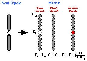 Figure 1: 3D dipole and load models
In order to determine the effect of the sensors on the total field, different
numbers of metallic sensors have been uniformly distributed on a circle and
illuminated by a unit plane wave at f=3GHz in free space.
The magnitude of the total field due to the unique presence of the sensors is represented
on Figure 2, for a number of sensors equal to 2, 4, 8, 32, 64 and 128.
We can clearly see the presence of the sensors, and also the perturbation they generate
with respect to the classical incident field (the unit plane wave).
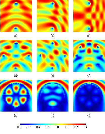 Figure 2: Magnitude of the total field with (a-c) 2, (d-e) 4, (f) 8, (g) 32, (h) 64, (i) 128 sensors, for a unit (a,d,f-i) vertical, (b,e) oblique or (c) horizontal plane wave
A test object, similar in terms of permittivity to a ceramic, is then positioned
at the center of the sensors network, in order to compare the field in this zone
compared to what it would have been without sensors.
The object, shown in Figure 3, has been discretized with 49 square cells of size
lambda/10, such that the total field inside the object
is correctly represented according to Hagmann's criterium.
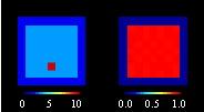 Figure 3: Test Object The magnitudes of the total field inside the object are represented on Figure 4 for the 2D sensor model and FIgure 5 for the 3D sensor model. An oblique plane incident wave at f=3GHz was used. The total field representation (a) and the scattered field one (c) are due to the object alone. The position and the square section of the object clearly appear on these figures, as does the shadow region it generates. This is a classical result, which does not take into account the perturbing presence of the sensors. The total field due to the object and the sensors is represented in (b). We can clearly observe the perturbation related to the sensors, and also their positions. On the other hand, the perturbation coming from the object is highly hidden. The only way to detect the presence of an object on the field patterns lies in the non symmetrical nature of the field with respect to the axis of the incident field. Finally, the total field due to the sensors alone is shown in (f).
When conducting an experiment, that is, when the measurement data
are real and not simulated,
the scattered field taken into account is the field obtained after the calibration
of the measurement system. Numerous calibration procedures exist. The simplest of these
and most commonly used consists in considering the difference between the measured scattered field
with object and the measured scattered field without object due to the unique
interactions between
sensors. The magnitude of this calibrated field is shown Figure 4(d) and (j).
The perturbation due to the sensors is still remarkable, but in a less pronounced
manner, and the position of the object can be localized, even though the field
is perturbed. The perturbation due to the sensors in free space is
therefore not neglectable.
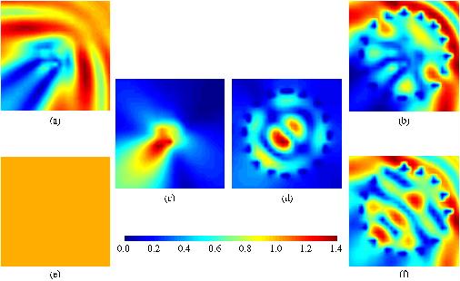 Figure 4: Magnitude representation of the total and calibrated fields: (a) (g) total field due to the object alone, (e) (k) incident field, (b) (h) total field due to the object and the 2D sensors, (d) (j) calibrated field, (c) (i) scattered field due to the object alone, (f) (l) total field due to the 2D sensors alone 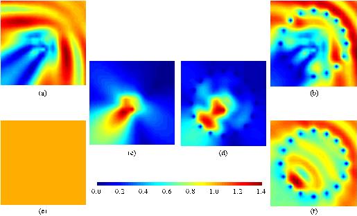 Figure 5: Magnitude representation of the total and calibrated fields: (a) (g) total field due to the object alone, (e) (k) incident field, (b) (h) total field due to the object and the 3D sensors, (d) (j) calibrated field, (c) (i) scattered field due to the object alone, (f) (l) total field due to the 3D sensors alone
Inverse Scattering Reconstructions
First, the classical algorithm has been used with the calibrated field
(Figure 6). The classical algorithm
diverges, which corroborates the necessity of developping the formal compensation
of sensors related interactions.
 Figure 6: Reconstruction with classical formalism. Slide your mouse on the image to see reconstruction animation.
Then, the algorithm with formal compensation has been used and converges as it can be seen
on Figure 7.
Figure 7: Reconstruction with formal compensation. Slide your mouse on the image to see reconstruction animation.
the advantage of introducing the sensors into the formalism appears to be
necessary as soon as the experiment is set in a lossless medium, as it is the
case for dielectric
characterization of composite material or high-resistance ceramics in free space.
Furthermore, the alibrated field cannot be considered as a satisfactory candidate for the
solving of the inverse problem.
Our new technique allows on the contrary to use the
Newton-Kantorovich reconstruction process coupled with the formal compensation
method to obtain very good reconstruction results
(convergence of the algorithm).
Experimental Modeling
The previous results have allowed to present the new method of formal compensation of sensors related interactions and to test the capacities of the new algorithms, but they cannot substitute real experimental measurements, which are the only ones to justify the real efficiency of a reconstruction process. Unfortunately there is no fully three-dimensional experimental system available today, even though measurement data are effectively three-dimensional (which implies the need of correcting anyhow these data to use them with two-dimensional algorithms).
First, experimental data from the 434Mhz microwave scanner developped at the
L.S.S. (Supelec, France)
have been used. These measurements have
been performed by Dr. J.-M. Geffrin duringhis Ph.D. thesis.
The 434Mhz scanner is a biomedical microwave imaging system.
It is composed of a metallic cuve filled with water and of radius a=29.5cm.
An external mecanical system directs two biconical antennas (one transmitter and
one receiver) inside the cuve.
A photograph of the system is given in Figure 8.
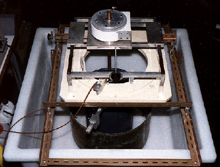 Figure 8: Photograph of the 434MHz scanner In his thesis, Dr. J.-M. Geffrin has taken into account the effects of the metallic cuve by computing the Green's function of a metallic circular cavity instead of using the free-space Green's function (as it is done here). Hence, the expression of the Green's function had to be evaluated numericly for all possible distances and was computed for this specific case. The cuve has been modeled in this thesis by small metallic sensors evenly distributed along a circle of the radius of the physical cuve. 200 contiguous sensors of radius r=0.23mm and conductivity sigma=10^6 S/m have been used, and the free-space Green's function has been kept.
The experimental data measurements have been performed with an homogeneous
cylindrical object of complex permittivity epsilon = (54.20,38.40) equivalent
to human muscle centered inside the system.
The object is illuminated by three different incident angles.
Thus, the measurement data is made of three series of 57 complex values
corresponding to the values of the scattered field for 57 position of the receiving
antenna (out of the 60 possible set in the simulation, for mecanical reasons), for
each of the 3 source positions.
The simulated scattered field values are compared on Figures 9 (magnitude)
and 10 (phase) with the experimental measurement data.
As it appears, the experimental data are fairly noisy with respect to the simulated data,
the quadratic error between the two being of about 30%, even though the model agrees
fairly well with the experiment.
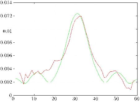 Figure 9: Magnitude of the simulated (green line) and experimental (dashed red line) scattered fields 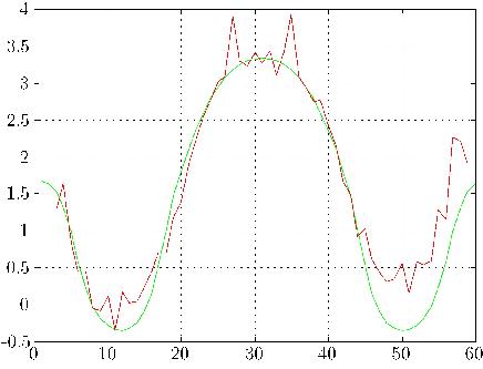 Figure 10: Phase (in gradients) of the simulated (green line) and experimental (dashed red line) scattered fields
Figure 11 shows the reconstructions obtained without a priori information
with an identity regularization procedure. The reconstruction results
with no a priori information, with
boundaries on the object's permittivity values, and a gradient-type regularization
associated to a regularization parameter computed with the cross-validation method
are shown in Figure 12.
From iteration 4, the algorithm converges towards the solution, the quadratic error on the
scattered field remaining around 30%.
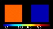 Figure 11: Reconstructions of the homogeneous cylinder with experimental data with no a priori information and identity regularization. Slide your mouse on the image to see reconstruction animation. Figure 12: Reconstructions of the homogeneous cylinder with experimental data with no a priori information and gradient regularization. Slide your mouse on the image to see reconstruction animation.
Second, the free-space dielectric characterization system from the
Genoa University (Italy)
has been modeled in order to process the experimental
data gathered by R. Azaro, S. Caorsi and M. Pastorino, and is still presently worked on.
The experimental system is made of a data acquisition device and a measuring system, shown
on Figures 13 and 14.
It uses the modulated scattering technique: an array of passive sensors
from which each dipole is successively modulated (through a diode) is mecanicly displaced
around the test area in front of a receiving antenna with a very large
aperture (ensuring a quasi uniform measurement).
The transmitting antenna is a dipole of size lambda/4 associated to
a plane reflector (at a distance of d=lambda/4
in order to generate an almost TM polarized incident wave.
The array is made of 27 printed circuits lambda/4 dipoles uniformly located on a
rectangular dielectric sheet of size 20cm-by-32cm and separated by a distance of
lambda/3.
Each dipole is successively loaded with a non-linear system in order to change the value of
its impedance and gather the measurement data.
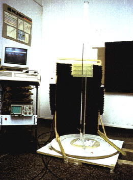 Figure 13: Photography of the experimental system 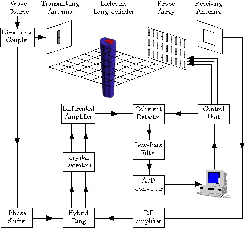 Figure 14: Diagram of the experimental system
For the experimental measurements, 3 different positions of the sensors array
have been used, as shown in Figure 15: on either side of the test
zone, and on the opposite side of it with respect to the source.
The test object is an infinitely long homogeneous cylinder of
square cross-section and real permittivity epsilon= 2.7, offset from the center
of the test area as shown on Figure 15.
The scattered field computed with the formal compensation method on the sensors
is presented on Figure 16, in comparison
with the scattered field simulated with the Genoa University model and the
measured scattered field.
It appears that the formal compensation method model allows the detection of the
measured discontinuity on sensor 8, which is not the case with the Genoa model.
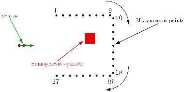 Figure 15: Geometry of the experimental system 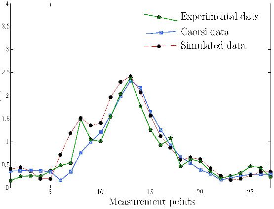 Figure 16: Magnitude of the scattered field on the sensors array
Conclusion
Numerical results lead us to the conclusion that sensors array related interactions are in many cases not neglectable in a lossless medium for dielectric chracterization applications. The introduction of the measurement sensors is therefore required in the reconstruction process if satisfactory results are seeked. The main objective of this research work has been to determine in which way all sensor related interactions could be formally taken into account in the microwave imaging algorithms. The experimental section enabled us to validate the modeling of a metallic ring for the forward problem; simulation results show good agreement with experimental results. As for the inverse problem, experimental data have been processed and, thank to a more complex regularization method, the object's permittivity values have been successfully reconstructed. The formal compensation's versatility gives the opportunity to model any arbitrary-shaped metallic cuve, without requiring preliminary computations like the Green's functions associated to the system, which could even be undetermined or not computable in the case of far too complex geometries. On the other hand, the modeling of the free-space 3GHz Genoa system has reached the goal of this thesis, that is, offer a new formal compensation of sensors related interactions, and it has shown that the sensors model accurately and faithfully simulates the interactions related to any particular experimental setup. The above work is a collaboration of Dr. Olivier Franza, Prof. J.-Ch. Bolomey, Dr. N. Joachimowicz, and Prof. Weng Cho Chew. Please send suggestions, comments, and inquiries to: olivier@sunchew.ece.uiuc.edu.
|