FASTANT
Overview
Fastant is an advanced antenna
simulation program developed under the direction of Professor Weng Cho Chew at
the Center for Computational Electromagnetics and Electromagnetics Laboratory
at the University of Illinois at Urbana Champaign. The volume-surface
integral equation is used to model various antennas in complex environments.
Using the Multilevel Fast Multipole Algorithm (MLFMA),1,2 Fastant can simulate very large problems, such as
antennas mounted on a car.
Fastant Examples
To illustrate the use of
Fastant, six examples are shown here.
Circular Microstrip Antenna
Figure 1 shows a top down view
of a circular microstrip antenna, with surface currents computed by Fastant.
The corresponding reflection coefficient and input impedance are shown in
Figure 2. The geometry and configuration of this simulation are stored in
the files microstrip.facet, microstrip.vol and microstrip.input.
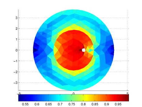
Figure 1: Current distribution of a circular
microstrip antenna.
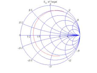
(a) Reflection coefficient
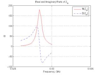
(b) Input impedance
Figure 2: Reflection coefficient and input
impedance of a circular microstrip antenna.
Dipole Antenna
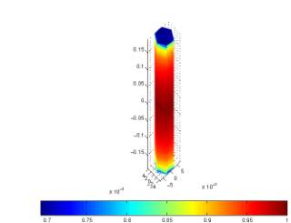
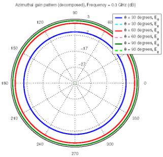
Figure 3(a) shows the current
distribution and geometry of a dipole antenna of length 0.375 m at an excitation frequency of 300 MHz. The
gain distribution associated with this antenna is shown in Figure 3(b).
With a hexagonal cross section,
the dipole was excited by six delta gap sources, one at the center of each
face. The potential of each source was fixed at 1 V. The excitation
frequency of these sources ranged between 300 and 450 MHz, at 10 MHz intervals.
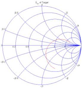
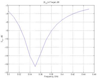
Figures 4 and 5 demonstrate the variation of the reflection coefficient
and input impedance as a function of excitation frequency.
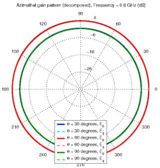
Observations of the radiated
field were made at polar angles θ = 30◦, θ = 60◦ and
θ = 90◦. Because Fastant expects the
elevation angle θe rather than the polar angle θ, one must remember that θe = 90◦ - θ.
The azimuthal angle θa =-f
ranged from 0◦ to 360◦
at intervals of 1◦.
There are 942 unknown current
elements in this simulation. Since this is a relatively small problem, Fastant
employed LU decomposition to invert the system matrix, rather than a fast
algorithm.
Being perfectly conducting, the antenna is completely
described by only the dipole.facet
and dipole.input files. The example archive
contains both of these files.
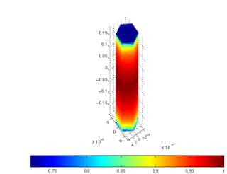
(a) Surface current
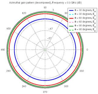
(b) Radiation gain
Figure 3: Surface current and radiation gain of a
dipole antenna at 300 MHz.
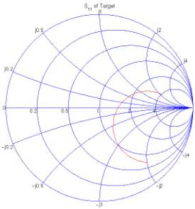
(a) Smith chart

(b) Rectangular axes
Figure 4: Reflection coefficient of a dipole
antenna at 300 MHz, on a Smith chart and on rectangular axes.
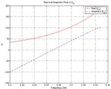
Figure 5: Input impedance of the dipole antenna
at 300 MHz.
Coated Dipole Antenna
The coated dipole antenna
consists of the dipole antenna described in the previous section, coated with a
2 mm thick layer of er =3.2
dielectric material. This material is modeled by 1,880 dielectric tetrahedra.
The metallic portions of the
antenna are described in coated.facet, which is identical to dipole.facet from the previous section. The
dielectric portions of the antenna are specified in coated.vol. The last file associated
with this simulation, coated.input, is substantially similar to dipole.input from the previous example.
However, Fastant must be told that there is one material which is not perfectly
conducting. In addition, the ICOAT value
must be set to some positive integer (which identifies the material in
the .vol file), the IBOUNDARY flag for the material must
be 3 (to tell Fastant that this is a dielectric material), and the dielectric
constant must be set to (3.2, 0.0).
The addition of a dielectric coating has pushed the
number of unknown current elements in this example to 5,318. A simulation of this size is still not
excessively large, so LU decomposition was once again chosen for inversion of
the system matrix. Figures 6, 7 and 8 show the results of this Fastant
simulation.
(a) Surface current
(b) Radiation gain
Figure 6: Surface current and radiation gain of a coated
dipole antenna at 300 MHz.
(a) Smith chart
(b) Rectangular axes
Figure 7: Reflection coefficient of a coated
dipole antenna at 300 MHz, on a Smith chart and on rectangular axes.
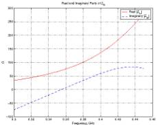
Figure 8: Input impedance of the coated dipole
antenna at 300 MHz.
Grounded Monopole Antenna
In this example, a 0.075 m monopole antenna is mounted on a 1 m ground
plane. As in the simple dipole example, this example is composed only of
perfect conductors, and requires only monopole.input and monopole.facet.
Simulations were conducted at 11
frequencies equally spaced between 800 MHz and 1.3 GHz, inclusive. Rather than rely on LU decomposition,
the system matrix was inverted with the GMRES iterative solver, accelerated by
MLFMA. The GMRES restart parameter was set to 100, and the method was limited
to 500 iterations. GMRES will terminate if the residual norm falls below 10−4 .
This problem is described by 2, 765 unknown current elements.
When using MLFMA, Fastant divides this problem into three levels at the lower
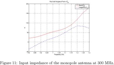
frequencies, and four levels at higher frequencies. Figures 9, 10 and 11 show
the results of the simulations.
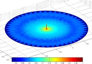
(a) Surface current
(b) Radiation gain
Figure 9: Surface current and radiation gain of a
monopole antenna at 300 MHz, over a ground plane.
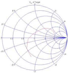
(a) Smith chart
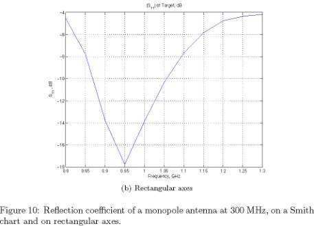
(b) Rectangular axes
Transmission Lines: Port Currents
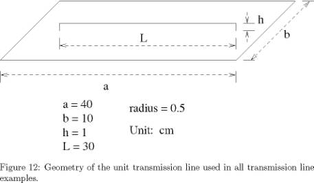
With the use of a .load input file, Fastant can
compute the currents passing through ports specified on a simulated
structure. To demonstrate this, consider the basic transmission line shown in
Figure 12. This line is used in three distinct simulations: a standalone line,
two parallel lines, and perpendicular sets of two parallel lines. Fastant was used
to calculate the currents on the lines and ground planes, in addition to the
port currents (specified at the ends of each line).
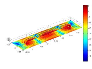
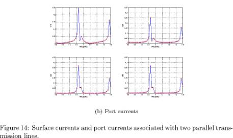
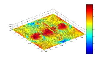
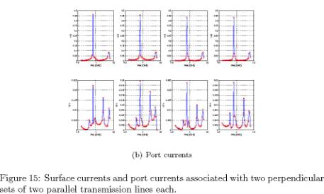
Figures 13, 14 and 15 show the
surface and port currents associated with one, two and four transmission lines,
respectively. These correspond to example files with base names of oneline, twolines and fourlines.
Each simulation requires .input, .facet, .vol, .wire and .load files
to produce the appropriate output.
Other parameters, such as input
impedance and reflection coefficient, are also calculated for each of
these examples. However, figures displaying these parameters have been
omitted. They may be reproduced using the example files distributed with
this manual.
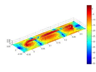
(a) Surface currents
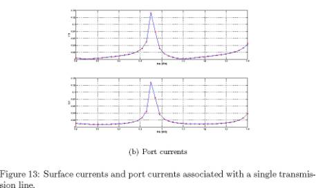
�.(b) Port currents
�.(a) Surface
currents
�.(b) Port currents
�.(a) Surface
currents
�.(b) Port currents
Isolated XM Antenna
In later examples, an XM antenna
is simulated in the presence of more complicated objects. It is thus useful to
examine the isolated antenna in detail. The bare XM antenna is shown with its surface
current distribution in Figure 16.
Fastant is also capable of
simulating the XM antenna when covered with a radome. Figure 17(a) shows the
current distributed excited on the radome. In Figure 17(b), the radome was
removed from the plot, showing the current distribution on the antenna in the
presence of the radome.
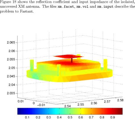
Figure 16: Current distribution
of an isolated XM antenna.
(a) Radome
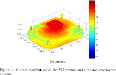
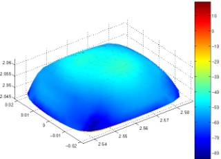
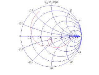
(b) Antenna (a) Reflection coefficient
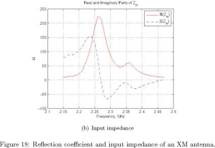
(b) Input impedance
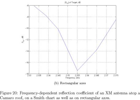
XM Antenna on a Camaro Roof
The first (and simplest)
of the complicated XM simulations places an XM antenna at the rear center of a
metallic Chevrolet Camaro roof. Because the structure has been extended
significantly, the number of unknown current elements has increased to
29,708, making this a substantial
problem. Figure 19 shows a view of the simulation geometry (with induced surface
currents) and the corresponding radiation patterns of the antenna roof
structure. The antenna structure shown in Figure 16 is located within the
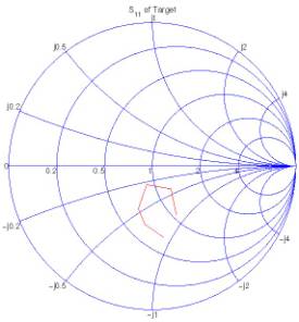
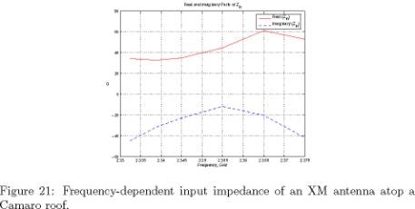
yellow ring on the roof. The reflection coefficient of the antenna is
plotted in Figure 20, while Figure 21 shows the antenna’s input impedance on
this structure. The basic Fastant input configuration and problem
geometry are described in the files roof.input, roof.facet
and roof.vol.
This example makes use of the self box interaction (SBI)
method to directly invert the portion of the system matrix corresponding to the
antenna. This results in increased accuracy at the center of activity of the
structure. The self box is described in the file roof.sbi.
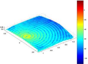
(a) Surface current
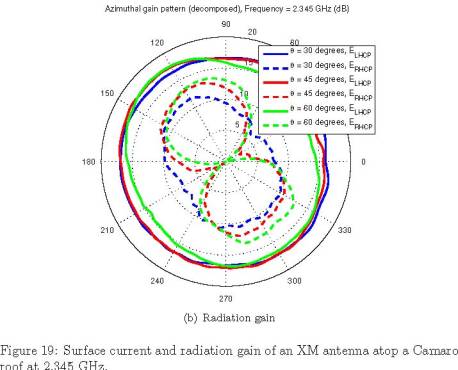
(b) Radiation gain
(a) Smith chart
�.(b) Rectangular
axes
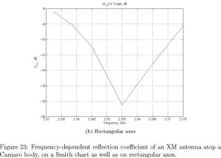
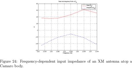
XM Antenna on a Camaro Body without Chassis
Extending the previous structure
further, this example details the simulation of an XM antenna on the roof of
the entire Camaro body. This structure contains neither the car’s chassis nor
its wheels. The number of unknown current elements in this problem has jumped
to 205,211. The induced currents and
corresponding radiation patterns are displayed in Figure 22. The
reflection coefficient and input impedance are shown in Figures 23 and
24, respectively.
The simulation files for this example are camaronc.input, camaronc.facet, camaronc.vol and camaronc.sbi.
Running this simulation will take several hours on a fast workstation.
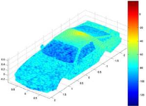
(a) Surface current
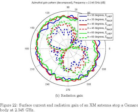
(b) Radiation gain
(a) Smith chart
�.(b) Rectangular
axes

XM Antenna on a Complete Camaro
Finally, the Camaro is completed
by adding a chassis and wheels. The XM antenna retains its position at the
rear of the roof. At a frequency of 2.345
GHz, this problem requires 508, 089
unknown current elements for each simulation. The memory required to simulate
the problem was in excess of 3.5 GB.
Because of the size and complexity of this simulation, it was only run for one
frequency. Consequently, frequency dependent plots of reflection coefficient
and input impedance are unavailable. Figure 25 shows the induced currents and
radiation patterns for this simulation.
The files camaro.input, camaro.facet, camaro.vol and camaro.sbi are
required by this example. This simulation may be expected to take twice as
long as the previous example. While the memory requirements may be prohibitive
on a typical desktop computer, this example is not a demanding task for a
supercomputer.
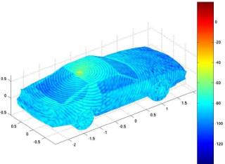
(a) Real surface current
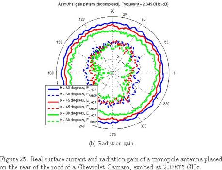
(b) Radiation gain
REFERENCES:
- Chao, HY; Chew, WC; Lu, CC: A
fast volumesurface integral equation
solver for radiation and scattering from wire antennas, impedance surfaces
and inhomogeneous dielectric objects. IEEE Antennas and Propagation Society International
Symposium (2002) 16–21.
- Chew, WC; Jin, JM; Michielssen, E; Song JM, Fast and Efficient Algorithms in Computational Electromagnetics, Artech House, MA, 2001.